no place to be ending but somewhere to start
Smoothing algorithms have a variety of applications from reducing short-term fluctuations in time series data, to forecasting, to edge detection and noise reduction in image processing. In this post, we’ll take a look at a group of smoothing algorithms available in traquer applied to time-series data.
some context
The following smoothing algorithms use Apple’s (AAPL) daily stock price over a roughly 6.5 year period as input. When applicable, a window size of 16 is used which is probably closer to the lower end of lookback lengths. In most cases, the suggested defaults (from Bing) of a algorithm are used. Yes, the hottest take in this post is Bing is better than Google at the time of writing (the author’s views may not reflect reality).
This post aims to highlight differences in behaviour between algorithms and does not intend to suggest which algorithms are best. Depending on use case, a flatter, smoother result may be desirable and in other cases, the opposite. Additionally, the post is subjective and should be questioned as the author has no statistical background, has not been in school for many years, and continues to refute the solution to the Monty Hall problem.
the basics
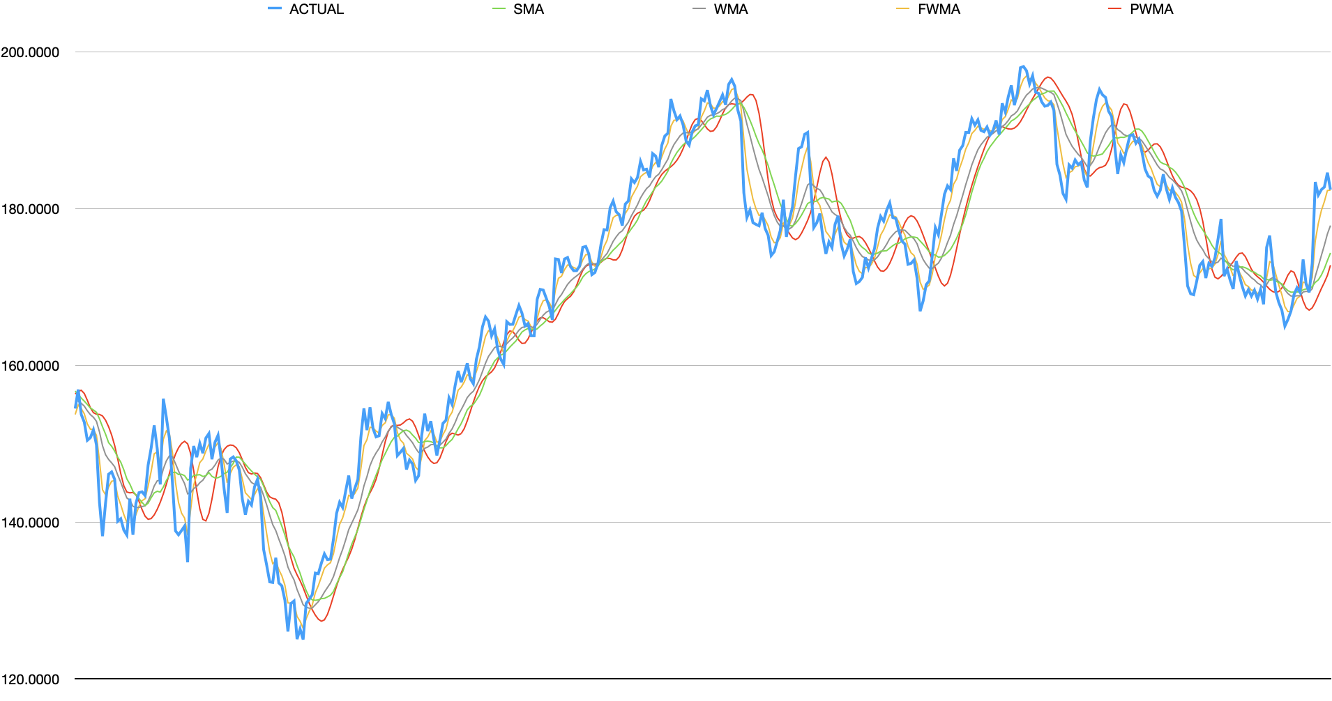
A common smoothing technique is to apply weights to each point across a window of values. These weights can be set to: treat all values in window equally; linearly place more weight on recent data or some other pattern. The first set of moving averages cover: Simple Moving Average (SMA), (linearly) Weighted Moving Average (WMA), Fibonacci Weighted Moving Average (FWMA), and Pascal’s Triangle Weighted Moving Average (PWMA).
analysis
- SMA - does a good reducing the noise but is not very responsive and lags
- WMA - does an equally good job reducing noise and is slightly more responsive than SMA (but still lags)
- FWMA - extremely responsive but arguably (extremely) noisy.
- PWMA - the least responsive but does better job at tracking short, but signicant spikes than SMA.
exponential and simple derivatives
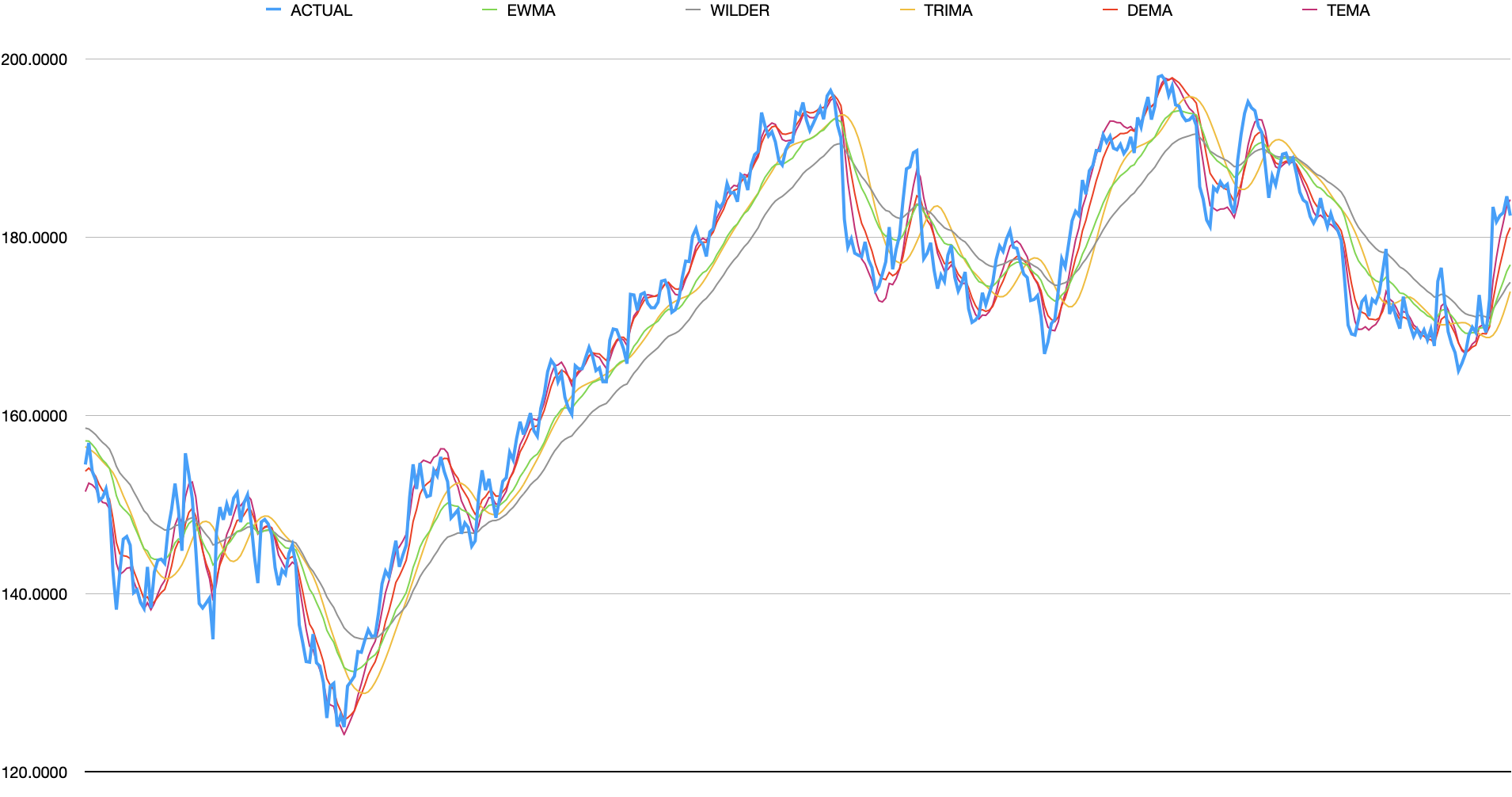
Rather than looking back a fixed length, another technique is to incrementally roll forward and combine the entire past with the new data. Exponential Weighted Moving Average (EWMA) and Wilder’s Moving Average (Wilder) leverage this technique. Additionally, applying these techniques multiple times can produce alternative smoothed data which is what Double Exponential Weighted (DEMA), Triple Exponential Weighted (TEMA), and Triangular Moving Average (TRIMA) do.
analysis
- EWMA - responsive but tends to lag when momentum increases
- Wilder - this technically produces the same results as EWMA but since the same window size is used in this case, lags more
- TRIMA - smoother but less responsive than SMA which it is based off of. similar to EWMA but does not flatten significant data as much
- DEMA - more responsive than EWMA with slightly more noise
- TEMA - similar responsiveness as DEMA but captures even more noise
1 + 1 = window
Beyond the moving average algorithms described above, alternative algorithms can be applied from simple techniques such as adding scaling factors or leveraging linear regression to applying Gaussian distributions and what can be described as “an equation formed by spilling a box of toothpicks on the floor.” These algorithms are broken in 3 arbitrary groups.
group 1
The following shows T3 Moving Average (T3), McGinley Dynamic Moving Average (MDMA), Hull’s Moving Average (HULL), and Zero Lag Moving Average (ZLMA).

analysis
- T3 - performs similarly to TRIMA but flattens minor peaks/valleys more while also capturing more of major peaks
- MDMA - similar responsiveness as T3, flattens data significantly more in general yet will still capture some minor spikes
- Hull - tracks input data very closely. only minor smoothing is present
- ZLMA - very similar to Hull with minutely more flattening.
group 2
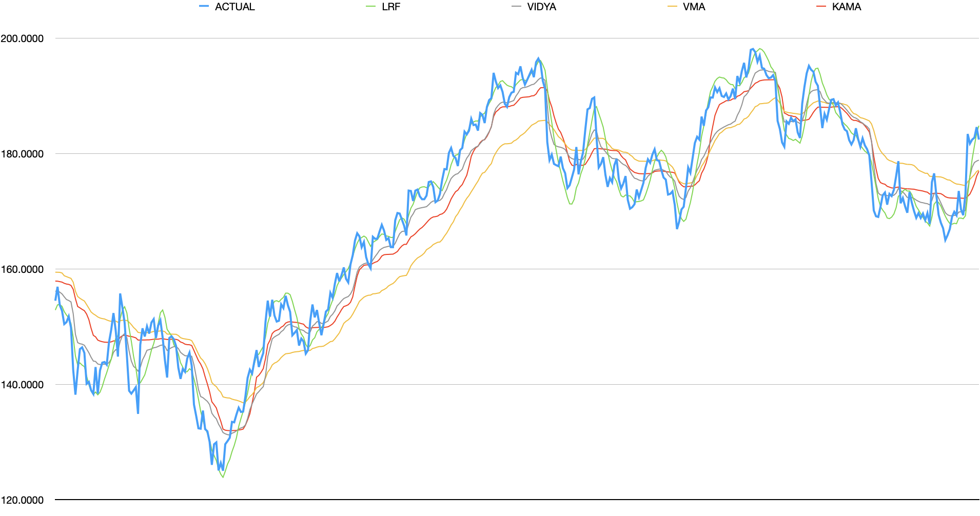
The next group consists of Linear Regression Forecast LRF, Volatility Index Dynamic Average (VIDYA), Variable Moving Average (VMA), and Kaufman Adaptive Moving Average (KAMA).
analysis
- LRF - similar to Hull’s MA but removes a little more noise
- VMA - unarguably produces the line least similar to original. both lags and flattens aggressively.
- KAMA - is slightly less responsive than most other algorithms. tends to flatten minor trends. while it flattens, contains jitter as if it drawn by an unsteady hand
- VIDYA - similar to KAMA but noisier
group3
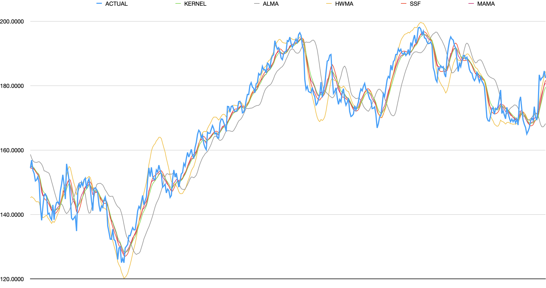
The last group contains algorithms with arguably the most novel designs, some of them inexplicable. These are: Kernel Regression (KERNEL), Arnaud Legoux Moving Average (ALMA), Holt-Winter Moving Average (HWMA), Super Smoother Filter (SSF), and MESA Adaptive Moving Average (MAMA).
It should be noted that the Kernel Regression algorithm is slightly modified from what is typically stated on internet. The implementation only tracks up to 255 datapoints and does not factor in future data. Therefore, it’s actually only apply half of the Gaussian curve.
analysis
- Kernel - responsive and flattens away most minor spikes. will still capture short, large spikes.
- ALMA - flattens minor changes but is significantly less responsive than peers. appears to put less weight on recent datapoints.
- HWMA - responsive. tends to follow momentum and will over-shoot strong upward/downward momentum
- SSF - performs similarly to Kernel algorithm but captures the value more closely on peaks/valley
- MAMA - also similar to Kernel but more responsive.
measurements
The following shows the difference between the smoothed data and the raw data. Mean Absolute Error (MAE) shows the average residual; Root Mean Squared Error (RMSE) shows similar measure but captures outliers better; Mean Directional Accuracy (MDA) captures how closes it matches direction changes and R-squared (RSQ) is the average R-squared value over 50 datapoint windows.
A higher MDA/RSQ and lower MAE/RMSE does not necessarily suggest a better line. It most likely implies the line contains more noise.
| ALGO | MAE | RMSE | MDA | RSQ | RUNTIME (us) |
|---|---|---|---|---|---|
| ACTUAL | 0.0000 | 0.0000 | 1.0000 | 1.0000 | |
| FWMA | 1.1653 | 1.6557 | 0.7002 | 0.9147 | 5.0735 |
| TEMA | 1.4368 | 2.0997 | 0.6131 | 0.8631 | 13.558 |
| ZLMA | 1.5841 | 2.3050 | 0.5973 | 0.8309 | 4.5029 |
| DEMA | 1.8107 | 2.5952 | 0.5745 | 0.7978 | 8.9601 |
| LRF | 1.7882 | 2.6150 | 0.5751 | 0.7987 | 10.636 |
| HULL | 1.8476 | 2.7010 | 0.5470 | 0.7820 | 12.586 |
| MAMA | 1.8615 | 2.7206 | 0.5669 | 0.8218 | 124.05 |
| SSF | 1.9658 | 2.7901 | 0.5377 | 0.7629 | 11.013 |
| KERNEL | 2.1897 | 3.0360 | 0.5354 | 0.7380 | 331.98 |
| WMA | 2.5509 | 3.4808 | 0.4962 | 0.6761 | 6.1506 |
| HWMA | 2.7944 | 3.8717 | 0.5359 | 0.6913 | 18.845 |
| EWMA | 2.9089 | 3.8791 | 0.5038 | 0.6554 | 3.9494 |
| VIDYA | 2.7790 | 4.0803 | 0.5132 | 0.7336 | 13.455 |
| MDMA | 3.3796 | 4.5220 | 0.5026 | 0.6145 | 19.092 |
| SMA | 3.4003 | 4.5472 | 0.4874 | 0.5301 | 3.8258 |
| TRIMA | 3.6072 | 4.8562 | 0.4769 | 0.4843 | 5.1022 |
| PWMA | 3.8432 | 5.2218 | 0.4833 | 0.4445 | 5.0097 |
| WILDER | 4.2392 | 5.5003 | 0.4868 | 0.5096 | 12.539 |
| KAMA | 3.8181 | 5.6028 | 0.4962 | 0.5792 | 6.0502 |
| T3 | 4.1574 | 5.6869 | 0.4699 | 0.4175 | 27.265 |
| VMA | 5.1780 | 6.7629 | 0.4863 | 0.5203 | 17.301 |
| ALMA | 5.1010 | 6.7661 | 0.4711 | 0.3427 | 8.1427 |
- Using MAMA’s default parameters, it would actually lead in all categories but it is arguably not smoothing enough. The above numbers and chart lowers MAMA’s alpha to 0.25 to match the alpha of EWMA with window of 16.
- runtime is in microseconds across ~1700 datapoints on a M1 Mac Mini.
conclusion
This post has no intention of declaring which algorithm performs the best. It is partially an exercise to validate whether the author’s usage of EWMA/Wilder is justified and partially a self-promotion of the traquer library. Keep in mind, these results use default values and each algorithm’s behaviour may change based on input settings.