numpy in the sky, i can go twice as high
In addition to storing time-based data efficiently, one of the main functions a time-series database provides is the ability to query over temporal data and compute statistics. In both cases, this involves summarising vast amounts of data either for storage or to provide a new view.
Working on Gnocchi – an open-source, time-series database that leverages cloud-based storage – the ability to group data and provide new statistical views on the grouped data represents a critical path in addition to the ability to read and write data.
At its conception, Gnocchi original leveraged Pandas to supply the logic behind grouping and aggregating data. Pandas is a fantastic Python toolkit that provides various data structures and functions to manipulate datasets and is ubiquitous among data scientists. With that said, over time we realised that Pandas was overkill in the context of Gnocchi’s aggregation workflow.
Moving away from Pandas, two alternatives were identified: SciPy and NumPy.
At its core, NumPy provides the ability to construct multidimensional arrays. In addition to that, it supports fast, vectorised array operations which is something used heavily in machine learning tools such as TensorFlow but also in Gnocchi. (yes, i’m very good at adding in hypewords that are completely unrelated… cough blockchain, autonomous vehicles, cloud cough)
Alternatively, SciPy extends NumPy and provides a collection of helper functions and tools often used in signal and image processing but also provides the ability to compute statistics over an array.
The following will highlight the gains Gnocchi achieved by moving towards a more tailored solution rather than using an all-purpose toolkit.
performance
To test the performance difference for handling time-series statistics in NumPy, SciPy, and Pandas, the following code was used:
import datetime
import functools

from gnocchi import carbonara
import numpy
import pandas

now = datetime.datetime.now()
times = numpy.array([numpy.datetime64(now) + numpy.timedelta64(i * 15, 's')
                     for i in numpy.arange(5760)])
values = numpy.random.rand(5760)

def round_timestamp(ts, freq):
    # function to group datapoints to specific window range
    # this is handled internally by carbonara.GroupedTimeSeries for numpy route
    return pandas.Timestamp((pandas.Timestamp(ts).value // freq) * freq)

# set of window sizes to group by
min_delta = numpy.timedelta64('60', 's')
hr_delta = numpy.timedelta64('3600', 's')
day_delta = numpy.timedelta64('86400', 's')
As a note, carbonara handles the time-series structure and logic in Gnocchi. I’m using pandas==0.22.0, scipy==1.0.0, numpy==1.13.3, with Gnocchi4.1 to test statistics with SciPy and master(2018.01.10) to test NumPy. The implementation code can be found in GitHub for exact details.
initialisation
First, we’ll start by timing how long it takes to initialise the required data structure:
timeit series = pandas.Series(values, times)
1000 loops, best of 3: 418 µs per loop

timeit np_series = numpy.empty(values.size, \
                               dtype=[('timestamps', '<datetime64[ns]'), \
                                      ('values', '<d')]); \
       np_series['timestamps'] = times; \
       np_series['values'] = values
10000 loops, best of 3: 85.8 µs per loop
Right off the bat, representing a basic time-series in NumPy is almost 5x more performant.
grouping
Next, to test grouping performance, we’ll group the 5760 time-value pairs three ways: by minute, which creates 1440 groups of 4 points each; by hour, which creates 24 groups of 240 points; and by day, which creates 2 groups of 2880 points.
# minute granularity, 1440 groups of 4 points
timeit pd_min_group = series.groupby(functools.partial(round_timestamp, \
                                                       freq=60*10e8))
10 loops, best of 3: 33.9 ms per loop

timeit np_min_group = carbonara.GroupedTimeSeries(np_series, min_delta)
1000 loops, best of 3: 380 µs per loop
Similarly, for the other granularities:
# hourly granularity, 24 groups of 240 points
timeit pd_min_group = series.groupby(functools.partial(round_timestamp, \
                                                       freq=3600*10e8))
10 loops, best of 3: 33.9 ms per loop

timeit np_hr_group = carbonara.GroupedTimeSeries(np_series, hr_delta)
1000 loops, best of 3: 326 µs per loop

# daily granularity, 2 groups of 2880 points
timeit pd_min_group = series.groupby(functools.partial(round_timestamp, \
                                                       freq=86400*10e8))
10 loops, best of 3: 33.8 ms per loop

timeit np_hr_group = carbonara.GroupedTimeSeries(np_series, day_delta)
1000 loops, best of 3: 325 µs per loop
In this scenario, we see consistent performance in both Pandas and NumPy regardless of grouping granularity. Also, regardless of granularity, using NumPy yields 100x performance. It should be noted, that Pandas is probably doing a lot more than NumPy to provide additional functionality. Keeping that in mind, the above benchmark should not be considered as a 1:1 comparison.
aggregation
Now let’s compare how each solution performs when computing statistical values for the groups.
mean
In all three solutions, the performance is relatively stable with the pure NumPy solution performing ~2.4x faster.
# pandas groupby aggregation
timeit pd_min_group.mean()
10000 loops, best of 3: 197 µs per loop
timeit pd_hr_group.mean()
10000 loops, best of 3: 187 µs per loop
timeit pd_day_group.mean()
10000 loops, best of 3: 188 µs per loop

# scipy-based carbonara
In [91]: timeit np_min_group.mean()
1000 loops, best of 3: 353 µs per loop
In [92]: timeit np_hr_group.mean()
1000 loops, best of 3: 278 µs per loop
In [93]: timeit np_day_group.mean()
1000 loops, best of 3: 277 µs per loop

# numpy-based carbonara
In [34]: timeit np_min_group.mean()
10000 loops, best of 3: 86 µs per loop
In [32]: timeit np_hr_group.mean()
10000 loops, best of 3: 77.1 µs per loop
In [33]: timeit np_day_group.mean()
10000 loops, best of 3: 78.7 µs per loop
last
NumPy shines when computing the last value of each group. possibly because of the indexing functionality of NumPy, it returns over 20x faster.
# pandas groupby aggregation
In [37]: timeit pd_min_group.last()
10000 loops, best of 3: 186 µs per loop
In [41]: timeit pd_hr_group.last()
10000 loops, best of 3: 173 µs per loop
In [42]: timeit pd_day_group.last()
10000 loops, best of 3: 172 µs per loop

# numpy-based carbonara (no scipy solution in Gnocchi)
timeit np_min_group.last()
10000 loops, best of 3: 29.2 µs per loop
timeit np_hr_group.last()
100000 loops, best of 3: 8.56 µs per loop
timeit np_day_group.last()
100000 loops, best of 3: 8.18 µs per loop
percentile
When computing the percentile of very few groups, SciPy performs the best. NumPy on the other hand performs consistently regardless of the number of groups and can perform over 400x and 70x better than Pandas and SciPy respectively.
# pandas groupby aggregation
timeit pd_min_group.quantile(0.95)
1 loop, best of 3: 514 ms per loop
timeit pd_hr_group.quantile(0.95)
100 loops, best of 3: 10.5 ms per loop
timeit pd_day_group.quantile(0.95)
100 loops, best of 3: 2.16 ms per loop

# scipy-based carbonara
timeit np_min_group.quantile(95)
10 loops, best of 3: 89.3 ms per loop
timeit np_hr_group.quantile(95)
100 loops, best of 3: 2.07 ms per loop
timeit np_day_group.quantile(95)
1000 loops, best of 3: 491 µs per loop

# numpy-based carbonara
timeit np_min_group.quantile(95)
1000 loops, best of 3: 1.23 ms per loop
timeit np_hr_group.quantile(95)
1000 loops, best of 3: 1.16 ms per loop
timeit np_day_group.quantile(95)
1000 loops, best of 3: 936 µs per loop
max
Max aggregate computation results were surprising as Pandas appears to do some black magic. Similar for min aggregation, Pandas outperformed NumPy and SciPy by a clean margin. Whatever Pandas is doing we need to port it to Gnocchi.
# pandas groupby aggregation
timeit pd_min_group.max()
1000 loops, best of 3: 231 µs per loop
timeit pd_hr_group.max()
10000 loops, best of 3: 188 µs per loop
timeit pd_day_group.max()
10000 loops, best of 3: 184 µs per loop

# scipy-based carbonara
timeit np_min_group.max()
1000 loops, best of 3: 887 µs per loop
timeit np_hr_group.max()
1000 loops, best of 3: 793 µs per loop
timeit np_day_group.max()
1000 loops, best of 3: 788 µs per loop

# numpy-based carbonara
timeit np_min_group.max()
1000 loops, best of 3: 559 µs per loop
timeit np_hr_group.max()
1000 loops, best of 3: 543 µs per loop
timeit np_day_group.max()
1000 loops, best of 3: 542 µs per loop
count
I’ll start off by saying this comparison is misleading af. In our carbonara group structure, count is computed on initialisation, so the NumPy solution is doing zero computation. With that said, it’s up to 55x faster. \o/
# pandas groupby aggregation
timeit pd_min_group.count()
10000 loops, best of 3: 157 µs per loop
timeit pd_hr_group.count()
10000 loops, best of 3: 165 µs per loop
timeit pd_day_group.count()
10000 loops, best of 3: 165 µs per loop

# numpy-based carbonara (no scipy solution in Gnocchi)
timeit np_min_group.count()
100000 loops, best of 3: 11.7 µs per loop
timeit np_hr_group.count()
100000 loops, best of 3: 3.12 µs per loop
timeit np_day_group.count()
100000 loops, best of 3: 2.94 µs per loop
multi-series aggregation
In this scenario, we’ll test how well each solution can aggregate across multiple independent time-series. We’ll use Gnocchi4.0 code to validate the Pandas solution (which may not be the best Pandas implementation) and master(2018.01.10) for NumPy (which also may not be the best NumPy implementation).
Without going too much into implementation details of Gnocchi, the Pandas solution takes multiple AggregatedTimeSerie (a Pandas series wrapped with supporting functions) and builds a Pandas DataFrame to do aggregation across the time-series collection. For the NumPy solution, we create similar AggregatedTimeSerie objects (a NumPy series wrapped with supporting functions) but rather than build a DataFrame, we build a AxB matrix where A is the number of series and B are the unique timestamps across all the series. the datasets are created as follows:
# gnocchi4.0 code
max_series = carbonara.AggregatedTimeSerie(60, "mean", pd_min_group.max())

# master(2018.01.10) code. each version was run separately, shown together
# for convenience
from gnocchi.rest.aggregates import processor
ref1 = processor.MetricReference(mock.Mock(id="metric1", name="metric1"),
                                 "mean", None)
ref2 = processor.MetricReference(mock.Mock(id="metric2", name="metric2"),
                                 "mean", None)
ref3 = processor.MetricReference(mock.Mock(id="metric3", name="metric3"),
                                 "mean", None)
max_series = carbonara.AggregatedTimeSerie(numpy.timedelta64('60', 's'),
                                           "mean", np_min_group.max())
Using this series, we’ll aggregate across 3 identical series, filling in missing values with 0 (although there are no missing values in this case):
# gnocchi4.0 code
timeit carbonara.AggregatedTimeSerie.aggregated([max_series, max_series, \
                                                 max_series], \
                                                aggregation="mean", \
                                                fill=0)
10 loops, best of 3: 28.8 ms per loop

# master(2018.01.10) code. each version was run separately, shown together
# for convenience
timeit processor.aggregated([(ref1, max_series), (ref2, max_series)], \
                             (ref3, max_series)], \
                            operations=["aggregate", "mean", \
                                        ["metric", "metric1", "metric2"]], \
                            fill=0)["aggregated"]
1000 loops, best of 3: 712 µs per loop
This is also done with the same 3 series except the holes are not filled. Note that the Pandas path is going to be much slower as significant parts of this logic are not in Pandas but in Python:
# gnocchi4.0 code
timeit carbonara.AggregatedTimeSerie.aggregated([max_series, max_series, \
                                                 max_series], \
                                                aggregation="mean")]
1 loop, best of 3: 734 ms per loop

# master(2018.01.10) code. each version was run separately, shown together
# for convenience
timeit processor.aggregated([(ref1, max_series), (ref2, max_series), \
                             (ref3, max_series)], \
                            operations=["aggregate", "mean", \
                                        ["metric", "metric1", "metric2", \
                                         "metric3"]])["aggregated"]
1000 loops, best of 3: 783 µs per loop
Reviewing the performance, by building the series in NumPy and maintaining the vast majority of logic and operations in NumPy, we are able to achieve up to 1000x performance gains in the above use case. This does not factor in the flexibility to perform vectorised mathematical operations across the series
There are more potential aggregates but they are consistent with above results. to be honest, i was actually expecting a greater performance gain compared to Pandas so i have to give props to the Pandas team for the continual improvements they’ve made! (or my benchmarks are wrong… or the code sucks)
memory
Personally, another reason for swapping out Pandas was to lower the memory requirements of each service so Gnocchi could run anywhere easily and reserve its memory for real work rather than to run Gnocchi. Pandas requires a non-trivial (for Python) amount of memory when loaded:
[fedora@gordcdev chungg.github.io]$ python -m memory_profiler /tmp/mem_prof
Filename: /tmp/mem_prof

Line #    Mem usage    Increment   Line Contents
================================================
     1   32.480 MiB   32.480 MiB   @profile
     2                             def load():
     3   64.484 MiB   32.004 MiB       import pandas  # pandas==0.22.0

[fedora@gordcdev chungg.github.io]$ python -m memory_profiler /tmp/mem_prof
Filename: /tmp/mem_prof

Line #    Mem usage    Increment   Line Contents
================================================
     1   32.574 MiB   32.574 MiB   @profile
     2                             def load():
     3   61.734 MiB   29.160 MiB       from scipy import ndimage  # scipy==1.0

[fedora@gordcdev chungg.github.io]$ python -m memory_profiler /tmp/mem_prof
Filename: /tmp/mem_prof

Line #    Mem usage    Increment   Line Contents
================================================
     1   32.676 MiB   32.676 MiB   @profile
     2                             def load():
     3   45.234 MiB   12.559 MiB       import numpy  # numpy==1.13.3
Depending on the packaged loaded, Pandas alone can be larger than 55MB. By swapping out Pandas for SciPy and then SciPy for NumPy, memory usage for Gnocchi’s processing workers drops more than 40%.
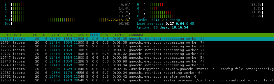 Gnocchi3 memory usage
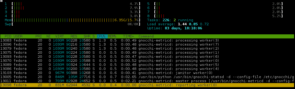 (almost) Gnocchi4.1 memory usage
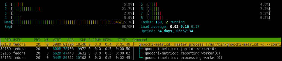 (potential) Gnocchi4.2 memory usage
end thought
By switching from Pandas to NumPy in Gnocchi, we were able to increase metric processing throughput and decrease memory usage. With all that said, Gnocchi does still require significant CPU but that’s maths for you.
revisions
- 2018-01-12: fixed some english; added more details to multi-series aggregate
- 2018-01-22: so you like capitals?