non-distributed dataframe shootout
Following up on my look into Vaex as an alternative to Pandas for building dataframes/tables in Python, this post will look at three more dataframe solutions. Polars is a relatively new solution built on Rust and Arrow with the eye-catching title of I wrote one of the fastest DataFrame libraries. This post will also take a look at the underlying technology Polars is based on and whether directly using Arrow is a good idea. Lastly, these dataframe solutions will be compared with datatable which is a solution based on the R implementation except it is written in C++ rather than C.
Each of the dataframe solutions have various use cases that may or may not overlap with another solution; Polars possibly offers memory protection while Vaex targets memory usage. This is in no way a recommendation for one over another but rather how each performs in a basic workflow. This post also doesn’t consider distributed dataframes like Dask and Spark as quite frankly i’ve never faced a scenario where i dealt with datasets that were 50GB+ that were not just unfiltered exports of a database or a bad join.
configuration
The following is the configuration the benchmarks were tested against. The absolute numbers will differ depending on CPU/disk and impact of virtualisation::
- Debian 10 in WSL2
- i5 laptop, 4 CPU, 16GB of memory
- Python 3.9.7
- pandas==1.3.2
- polars==0.9.3
- pyarrow==5.0.0
- datatable==1.0.0
- vaex==4.4.0
In all test cases below, the timings shown for each case show the action performed in the following order:
- Pandas
- Polars
- PyArrow
- datatable
- Vaex
data
Below is the schema of the dataframe being used.
Business Date: date
Type1: string
Type2: string
Portfolio Code: string
Issuer: string
Metric1: double
Metric2: double
Fx Rate: double
Country: string
Metric3: double
Metric4: double
Parent Type1: string
Parent Group: string
Parent Type2: string
Group1: string
Group2: string
Group3: string
Group4: string
Metric5: int64
Days to Maturity: double
Type3: string
Underlying: string
Industy: string
Issue Date: date
ID1: string
Currency: string
Maturity Date: int64
Parent Name: string
Metric6: double
Group5: string
Region: string
Group7: string
Group8: string
Metric7: double
Metric8: double
Group9: double
Group10: string
Group11: string
Group12: string
Group13: string
Group14: string
Metric9: double
Group15: string
Metric10: double
It is based off a real dataset with 1219467 rows and 44 columns. As:
- csv, it is 465MB
- Parquet, it is 35MB.
- feather (Arrow IPC), it is 164MB (with default LZ4 compression)
memory
This is a crude test but to gauge memory footprint of each solution, i’m just importing the base package and noting the affect it has on resident memory in htop.
import pandas     # ~69MB
import polars     # ~79MB
import pyarrow    # ~44MB
import datatable  # ~6MB
import vaex       # ~110MB
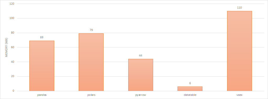 dataframe library memory footprint
To capture how much memory each library consumes to represent a dataframe, i’ve again captured the delta between the resident memory before and after reading the csv file. This doesn’t necessarily reflect exactly how much memory each solution needs as Pandas and Arrow both seem to use a few hundred megabytes more than what it eventually settled at and what is shown in the chart below.
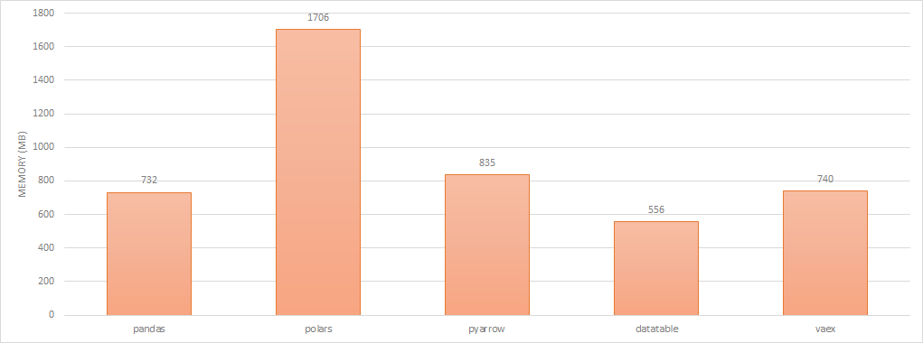 dataframe memory footprint
read
csv
# pandas
%timeit pd.read_csv('/tmp/test.csv')
6.07 s ± 374 ms per loop (mean ± std. dev. of 7 runs, 1 loop each)

# polars
%timeit pl.read_csv('/tmp/test.csv')
835 ms ± 21.6 ms per loop (mean ± std. dev. of 7 runs, 1 loop each)

# pyarrow
%timeit pa.csv.read_csv('/tmp/test.csv')
589 ms ± 19.1 ms per loop (mean ± std. dev. of 7 runs, 1 loop each)

# datatable
%timeit dt.fread('/tmp/test.csv')
1.36 s ± 101 ms per loop (mean ± std. dev. of 7 runs, 1 loop each)

# vaex
%timeit vaex.open('/tmp/test.csv')
10.1 s ± 895 ms per loop (mean ± std. dev. of 7 runs, 1 loop each)
When loading csv files, Polars, PyArrow, and datatable seem to saturate all cores.
parquet
%timeit pd.read_parquet('/tmp/test.parquet')
958 ms ± 16.3 ms per loop (mean ± std. dev. of 7 runs, 1 loop each)

%timeit pl.read_parquet('/tmp/test.parquet')
576 ms ± 73.5 ms per loop (mean ± std. dev. of 7 runs, 1 loop each)

%timeit pa.parquet.read_table('/tmp/test.parquet')
347 ms ± 14.3 ms per loop (mean ± std. dev. of 7 runs, 1 loop each)

# datatable does not support parquet files. Solution appears to be something like:
%timeit dt.Frame(pq.read_table('/tmp/test.parquet').to_pandas())
2.69 s ± 108 ms per loop (mean ± std. dev. of 7 runs, 1 loop each)

%timeit df = vaex.open('/tmp/test.parquet')
2.43 ms ± 44.4 µs per loop (mean ± std. dev. of 7 runs, 100 loops each)
arrow ipc
%timeit pd.read_feather('/tmp/test.feather')
766 ms ± 31.3 ms per loop (mean ± std. dev. of 7 runs, 1 loop each)

%timeit pl.read_ipc('/tmp/test.feather')
476 ms ± 85.8 ms per loop (mean ± std. dev. of 7 runs, 1 loop each)

%timeit pa.read_table('/tmp/test.feather')
146 ms ± 6.57 ms per loop (mean ± std. dev. of 7 runs, 10 loops each)

# datatable does not support arrow files. Solution appears to be something like below
# but it doesn't seem to generate correctly:
%timeit dt.Frame(pd.read_feather('/tmp/test.feather'))
2.15 s ± 41.1 ms per loop (mean ± std. dev. of 7 runs, 1 loop each)

%timeit vaex.open('/tmp/test.feather')
189 ms ± 39.5 ms per loop (mean ± std. dev. of 7 runs, 1 loop each)
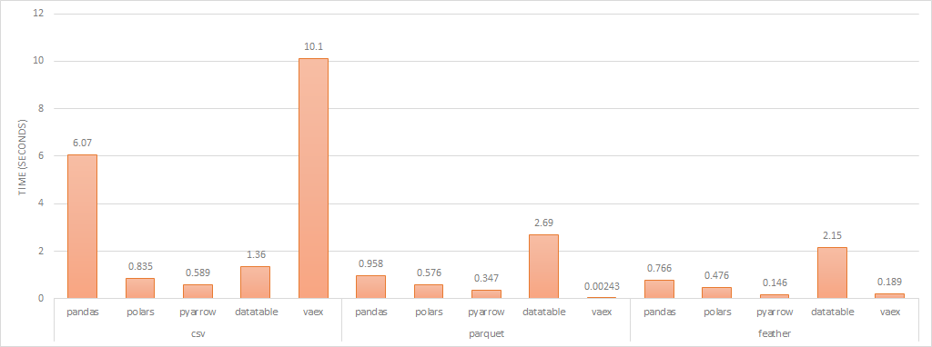 read performance (lower is better)
When loading Feather and Parquet files, all libraries used multiple cores to load. Vaex is lazy loaded which is why its load time is so much quicker compared to the others. It should also be noted, that you can filter on load, which reduces memory requirements and the need for distributed dataframe solutions.
aggregation
In all cases below, Pandas and PyArrow did not seem to use multiple cores to compute. For Polars and datatable, in some cases it seemed to saturate all cores and in others, only one. For Vaex, it appeared to use all cores but only one would actually be used fully.
mean
%timeit df['Metric1'].mean()
4.61 ms ± 141 µs per loop (mean ± std. dev. of 7 runs, 100 loops each)

%timeit df['Metric1'].mean()
600 µs ± 7.18 µs per loop (mean ± std. dev. of 7 runs, 1000 loops each)

%timeit pa.compute.mean(df['Metric1'])
770 µs ± 26.4 µs per loop (mean ± std. dev. of 7 runs, 1000 loops each)

%timeit df[:, 'Metric1'].mean()
2.26 µs ± 108 ns per loop (mean ± std. dev. of 7 runs, 100000 loops each)

%timeit df['Metric1'].mean()
351 ms ± 6.16 ms per loop (mean ± std. dev. of 7 runs, 1 loop each)
median
%timeit df['Metric1'].median()
20.2 ms ± 265 µs per loop (mean ± std. dev. of 7 runs, 10 loops each)

%timeit df['Metric1'].median()  # appeared to be multicore
33.5 ms ± 569 µs per loop (mean ± std. dev. of 7 runs, 10 loops each)

%timeit pa.compute.quantile(df['Metric1'])
13.4 ms ± 644 µs per loop (mean ± std. dev. of 7 runs, 100 loops each)

%timeit df[:, dt.median(f['Metric1'])]  # appeared to be multicore
38.7 ms ± 1.96 ms per loop (mean ± std. dev. of 7 runs, 10 loops each)

# Not supported in Vaex
value_counts
%timeit df['Group1'].value_counts()
34.3 ms ± 132 µs per loop (mean ± std. dev. of 7 runs, 10 loops each)

%timeit df['Group1'].value_counts()  # appeared to be multicore
20.2 ms ± 512 µs per loop (mean ± std. dev. of 7 runs, 10 loops each)

%timeit df['Group1'].value_counts()
11.8 ms ± 267 µs per loop (mean ± std. dev. of 7 runs, 100 loops each)

%timeit df[:, dt.count(f['Group1']), dt.by('Group1')]  # appeared to be multicore
93.3 ms ± 8.9 ms per loop (mean ± std. dev. of 7 runs, 10 loops each)

%timeit df['Group1'].value_counts()
132 ms ± 4.4 ms per loop (mean ± std. dev. of 7 runs, 10 loops each)
max
%timeit df['Metric1'].max()
4.52 ms ± 133 µs per loop (mean ± std. dev. of 7 runs, 100 loops each)

%timeit df['Metric1'].max()
3.38 ms ± 92.4 µs per loop (mean ± std. dev. of 7 runs, 100 loops each)

%timeit pa.compute.min_max(df['Metric1'])
4.4 ms ± 107 µs per loop (mean ± std. dev. of 7 runs, 100 loops each)

%timeit df[:, 'Metric1'].max()
2.42 µs ± 108 ns per loop (mean ± std. dev. of 7 runs, 100000 loops each)

%timeit df['Metric1'].max()
178 ms ± 2.76 ms per loop (mean ± std. dev. of 7 runs, 1 loop each)
std
%timeit df['Metric1'].std()
11.6 ms ± 192 µs per loop (mean ± std. dev. of 7 runs, 100 loops each)

%timeit df['Metric1'].std()
8.33 ms ± 271 µs per loop (mean ± std. dev. of 7 runs, 100 loops each)

%timeit pa.compute.stddev(df['Metric1'])
1.66 ms ± 22.6 µs per loop (mean ± std. dev. of 7 runs, 1000 loops each)

%timeit df[:, 'Metric1'].sd()
2.33 µs ± 143 ns per loop (mean ± std. dev. of 7 runs, 100000 loops each)

%timeit df['Metric1'].std()
558 ms ± 15.7 ms per loop (mean ± std. dev. of 7 runs, 1 loop each)
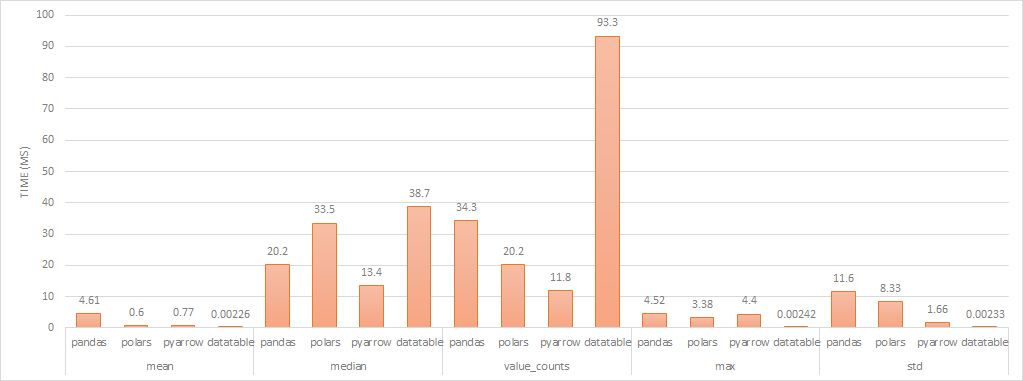 aggregate performance (lower is better)
I’ve removed Vaex from the chart as its performance is magnitudes slower than the others and would hide any differences. datatable performs much faster than the other libraries in some cases but at a speed that makes me think that the aggregation is precomputed and is effectively doing a lookup when the aggregation is requested. When aggregations do utilise the CPU, in most cases, Arrow performs the quickest but there are scenarios where Pandas and/or Polars performs comparably.
filter
single column - small resultset (52422 rows, ~5% of table)
%timeit df[df['Group1'] == 'AAA']
61.6 ms ± 854 µs per loop (mean ± std. dev. of 7 runs, 10 loops each)

%timeit df[df['Group1'] == 'AAA']
22.7 ms ± 718 µs per loop (mean ± std. dev. of 7 runs, 10 loops each)

%timeit df.filter(pa.compute.equal(df['Group1'], 'AAA'))
22.5 ms ± 483 µs per loop (mean ± std. dev. of 7 runs, 10 loops each)

%timeit df[f['Group1'] == 'AAA', :]
38 ms ± 2.32 ms per loop (mean ± std. dev. of 7 runs, 10 loops each)

%timeit df[df['Group1'] == 'AAA']
29 ms ± 999 µs per loop (mean ± std. dev. of 7 runs, 10 loops each)
single column - large resultset (652725 rows, ~55% of table)
%timeit df[df['Group1'] == 'CCC']
215 ms ± 2.15 ms per loop (mean ± std. dev. of 7 runs, 1 loop each)

%timeit df[df['Group1'] == 'CCC']
238 ms ± 6.94 ms per loop (mean ± std. dev. of 7 runs, 1 loop each)

%timeit df.filter(pa.compute.equal(df['Group1'], 'CCC'))
150 ms ± 7.82 ms per loop (mean ± std. dev. of 7 runs, 1 loop each)

%timeit df[f['Group1'] == 'BBB', :]
40.5 ms ± 1.14 ms per loop (mean ± std. dev. of 7 runs, 10 loops each)

%timeit df[df['Group1'] == 'CCC']
28.4 ms ± 423 µs per loop (mean ± std. dev. of 7 runs, 10 loops each)
single column, multiple conditions - small resultset (75105 rows, ~5% of table)
%timeit df[(df['Group1'] == 'AAA') | (df['Group1'] == 'BBB')]
116 ms ± 1.15 ms per loop (mean ± std. dev. of 7 runs, 10 loops each)

%timeit df[(df['Group1'] == 'AAA') | (df['Group1'] == 'BBB')]
35.1 ms ± 385 µs per loop (mean ± std. dev. of 7 runs, 10 loops each)

%timeit df.filter(pa.compute.or_(pa.compute.equal(df['Group1'], 'AAA'),
                                 pa.compute.equal(df['Group1'], 'BBB')))
35.6 ms ± 638 µs per loop (mean ± std. dev. of 7 runs, 10 loops each)

%timeit df[(f['Group1'] == 'AAA') | (f['Group1'] == 'CCC'), :]
62.3 ms ± 1.41 ms per loop (mean ± std. dev. of 7 runs, 10 loops each)

%timeit df[(df['Group1'] == 'AAA') | (df['Group1'] == 'BBB')]
87.7 ms ± 1.65 ms per loop (mean ± std. dev. of 7 runs, 10 loops each)
single column, multiple conditions - large resultset (675408 rows, ~55% of table)
%timeit df[(df['Group1'] == 'CCC') | (df['Group1'] == 'BBB')]
306 ms ± 17.9 ms per loop (mean ± std. dev. of 7 runs, 1 loop each)

%timeit df[(df['Group1'] == 'CCC') | (df['Group1'] == 'BBB')]
271 ms ± 9.05 ms per loop (mean ± std. dev. of 7 runs, 1 loop each)

%timeit df.filter(pa.compute.or_(pa.compute.equal(df['Group1'], 'CCC'),
                                 pa.compute.equal(df['Group1'], 'BBB')))
154 ms ± 8.93 ms per loop (mean ± std. dev. of 7 runs, 1 loop each)

%timeit df[(f['Group1'] == 'BBB') | (f['Group1'] == 'CCC'), :]
56.1 ms ± 2.37 ms per loop (mean ± std. dev. of 7 runs, 10 loops each)

%timeit df[(df['Group1'] == 'CCC') | (df['Group1'] == 'BBB')]
86.1 ms ± 1.01 ms per loop (mean ± std. dev. of 7 runs, 10 loops each)
single column, “in” condition (75105 rows, ~5% of table)
%timeit df[df['Group1'].isin(['AAA', 'BBB'])]
41.8 ms ± 665 µs per loop (mean ± std. dev. of 7 runs, 10 loops each)

%timeit df[df['Group1'].is_in(['AAA', 'BBB'])]
43.4 ms ± 716 µs per loop (mean ± std. dev. of 7 runs, 10 loops each)

%timeit df.filter(pa.compute.is_in(df['Group1'], value_set=pa.array(['AAA', 'BBB'])))
33.8 ms ± 990 µs per loop (mean ± std. dev. of 7 runs, 10 loops each)

# not applicable in datatable, need to chain with or

%timeit df[df['Group1'].isin(['AAA', 'BBB'])]
30.6 ms ± 634 µs per loop (mean ± std. dev. of 7 runs, 10 loops each)
multiple columns - small resultset (9708 rows, ~1% of table)
%timeit df[(df['Group1'] == 'AAA') & (df['Group2'] == 'Y')]
94.3 ms ± 811 µs per loop (mean ± std. dev. of 7 runs, 10 loops each)

%timeit df[(df['Group1'] == 'AAA') & (df['Group2'] == 'Y')]
10.5 ms ± 100 µs per loop (mean ± std. dev. of 7 runs, 100 loops each)

%timeit df.filter(pa.compute.and_(pa.compute.equal(df['Group1'], 'AAA'),
                                  pa.compute.equal(df['Group2'], 'Y')))
12.7 ms ± 133 µs per loop (mean ± std. dev. of 7 runs, 100 loops each)

%timeit df[(f['Group1'] == 'AAA') & (f['Group2'] == 'Y'), :]
39.2 ms ± 1.09 ms per loop (mean ± std. dev. of 7 runs, 10 loops each)

%timeit df[(df['Group1'] == 'AAA') & (df['Group2'] == 'Y')]
80.3 ms ± 2.08 ms per loop (mean ± std. dev. of 7 runs, 10 loops each)
multiple columns - large resultset (646188 rows, ~55% of table)
%timeit df[(df['Group1'] == 'CCC') & (df['Group2'] == 'N')]
284 ms ± 12.2 ms per loop (mean ± std. dev. of 7 runs, 1 loop each)

%timeit df[(df['Group1'] == 'CCC') & (df['Group2'] == 'N')]
243 ms ± 10.7 ms per loop (mean ± std. dev. of 7 runs, 1 loop each)

%timeit df.filter(pa.compute.and_(pa.compute.equal(df['Group1'], 'CCC'),
                                  pa.compute.equal(df['Group2'], 'N')))
150 ms ± 18.6 ms per loop (mean ± std. dev. of 7 runs, 1 loop each)

%timeit df[(f['Group1'] == 'BBB') & (f['Group2'] == 'N'), :]
56.5 ms ± 5.06 ms per loop (mean ± std. dev. of 7 runs, 10 loops each)

%timeit df[(df['Group1'] == 'CCC') & (df['Group2'] == 'N')]
81 ms ± 1.68 ms per loop (mean ± std. dev. of 7 runs, 10 loops each)
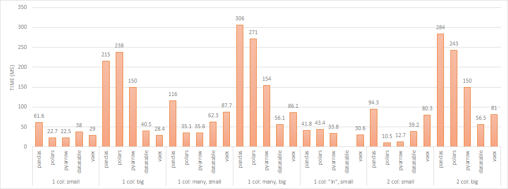 filter performance (lower is better)
In general, Arrow and Polars perform comparably when the result set is a small subset of the original table. Vaex and datatable perform similarly regardless of the size of the result set so there is probably a component of the operation that is lazily evaluated.
write
csv
%timeit df.to_csv('/tmp/test.csv')
20.7 s ± 770 ms per loop (mean ± std. dev. of 7 runs, 1 loop each)

%timeit df.to_csv('/tmp/test.csv')
3.45 s ± 202 ms per loop (mean ± std. dev. of 7 runs, 1 loop each)

# pyarrow using 6.0.0 to avoid https://issues.apache.org/jira/browse/ARROW-12540
%timeit pa.csv.write_csv(df, '/tmp/test.csv')
2.5 s ± 249 ms per loop (mean ± std. dev. of 7 runs, 1 loop each)

# datatable does not seem to offer ability to write

%timeit df.export_csv('/tmp/test.csv')
23.1 s ± 563 ms per loop (mean ± std. dev. of 7 runs, 1 loop each)
parquet
%timeit df.to_parquet('/tmp/test.parquet')
2.21 s ± 52.2 ms per loop (mean ± std. dev. of 7 runs, 1 loop each)

%timeit df.to_parquet('/tmp/test.parquet')
1.34 s ± 89 ms per loop (mean ± std. dev. of 7 runs, 1 loop each)

%timeit pa.parquet.write_table(df, '/tmp/test.parquet')
1.29 s ± 16.4 ms per loop (mean ± std. dev. of 7 runs, 1 loop each)

# datatable does not seem to offer ability to write

%timeit df.export_parquet('/tmp/test.parquet')
2.05 s ± 24.6 ms per loop (mean ± std. dev. of 7 runs, 1 loop each)
arrow ipc
%timeit df.to_feather('/tmp/test.feather')
1.26 s ± 87.5 ms per loop (mean ± std. dev. of 7 runs, 1 loop each)

# polars appears to write an uncompressed, possibly v1, arrow file
%timeit df.to_ipc('/tmp/test.feather')
2.68 s ± 487 ms per loop (mean ± std. dev. of 7 runs, 1 loop each)

%timeit pa.feather.write_feather(df, '/tmp/test.feather')
294 ms ± 9.52 ms per loop (mean ± std. dev. of 7 runs, 1 loop each)

# datatable does not seem to offer ability to write

%timeit df.export_feather('/tmp/test.feather')
294 ms ± 8.55 ms per loop (mean ± std. dev. of 7 runs, 1 loop each)
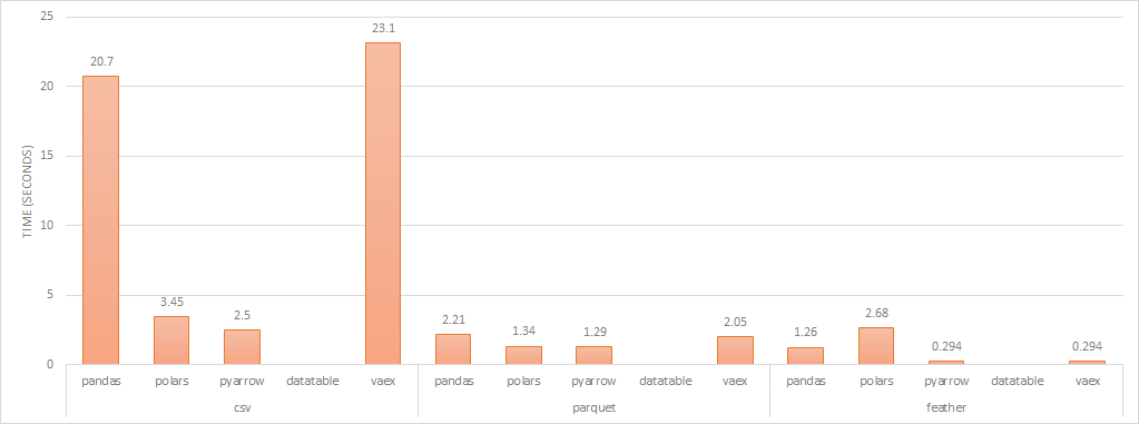 write performance (lower is better)
Writing to disk in csv, Polars performs markedly better than Pandas and Vaex but when writing as a binary file, all libraries perform similarly.
conclusion
Arrow offers a small, performant solution for handling dataframes in Python. It also visually, did not seem to saturate all the cores for many of the tasks which may allow for better parallelisation if where you run the computation is not memory constrained. That said, its syntax is significantly different from Pandas and NumPY, which Polars and Vaex mimic, so Polars might be a potential alternative if you already have Pandas-like code.
If you are memory constrained, Vaex is the only solution which by default lazy loads data but you can also conserve memory using Polars and Arrow by explicitly selecting columns which also improves read performance. datatable does a good job of memory usage if you blindly want to load the entire dataset.
Ultimately, regardless of the dataframe library chosen, storing tabular data in a binary format like Arrow IPC or Parquet will net the biggest performance gains as serialisation represents the vast majority of time spent when processing data. Arrow IPC generally has better performance but is currently less supported by third party services
revisions
- 2021-09-21: include datatable library
- 2021-11-05: include feather/arrow ipc file format